The discrete wavelet transform (DWT) is an implementation of the wavelet transform using a discrete set of the wavelet scales and translations obeying some defined rules. In other words, this transform decomposes the signal into mutually orthogonal set of wavelets, which is the main difference from the continuous wavelet transform (CWT), or its implementation for the discrete time series sometimes called discrete-time continuous wavelet transform (DT-CWT).
The wavelet can be constructed from a scaling function which describes its scaling properties. The restriction that the scaling functions must be orthogonal to its discrete translations implies some mathematical conditions on them which are mentioned everywhere e. g. the dilation equation
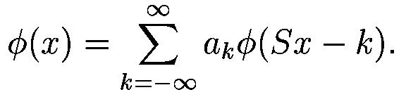
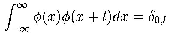
where S is a scaling factor (usually chosen as 2). Moreover, the area between the function must be normalized and scaling function must be ortogonal to its integer translates e. g.
After introducing some more conditions (as the resstrictions above soes not produce unique solution) we can obtain results of all this equations, e. g. finite set of coefficients a_k which define the scaling function and also the wavelet. The wavelet is obtained from the scaling function as
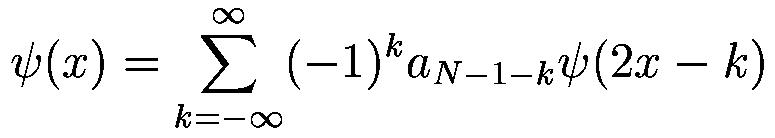
where N is an even integer. The set of wavelets than forms an orthonormal basis which we use to decompose signal. Note that usually only few of the coefficients a_k are nonzero which simplifies the calculations.
|
|
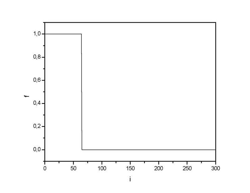
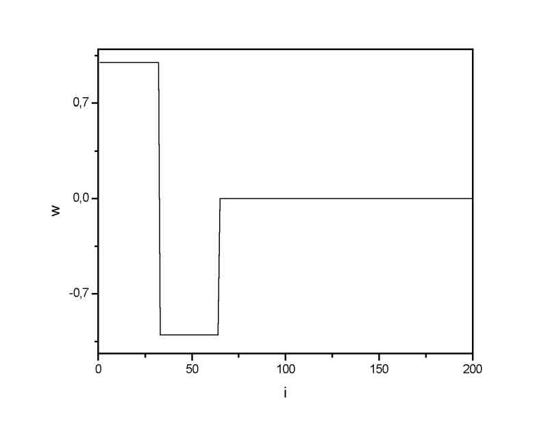
| Haar scaling function. | Haar wavelet. |
 |
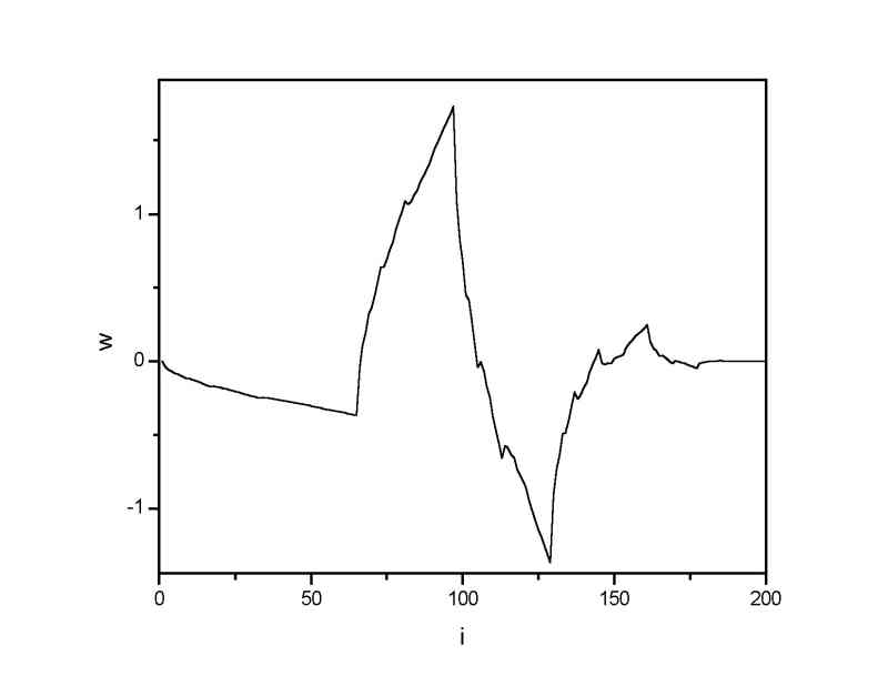 |
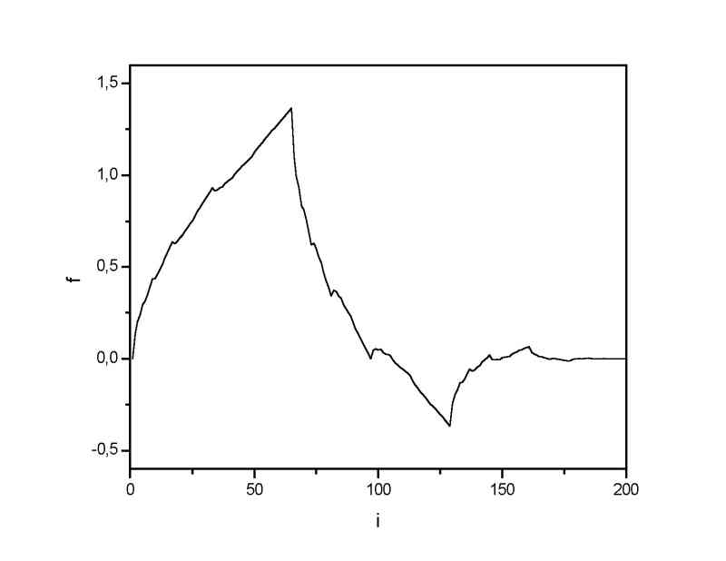
| Daubechies 4 scaling function. | Daubechies 4 wavelet. |
 |
 |
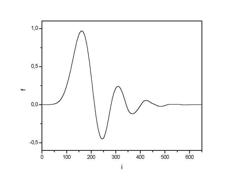
| Daubechies 20 scaling function. | Daubechies 20 wavelet. |
There are several types of implementation of the DWT algorithm. The oldest and most known one is the Malaat (pyramidal) algoritm. In this algorithm two filters - smoothing and non-smoothing one are constructed from the wavelet coefficients and those filters are recurrently used to obtain data for all the scales. If the total number of data D=2^N is used and signal length is L, first D/2 data at scale L/2^(N-1) are computed, than (D/2)/2 data at scale L/2^(N-2), ... etc up to finally obtaining 2 data at scale L/2. The result of this algorithm is an array of the same length as the input one, where the data are usually sorted from the largest scales to the smallest ones.
Similarily the inverse DWT can reconstruct the original signal from the wavelet spactrum. Note that the wavelet that is used as a base for decomposition can not be changed if we want to reconstruct the original signal, e. g. by using Haar wavelet we obtain a wavelet spectrum; it can be used for signal reconstruction using the same (Haar) wavelet.
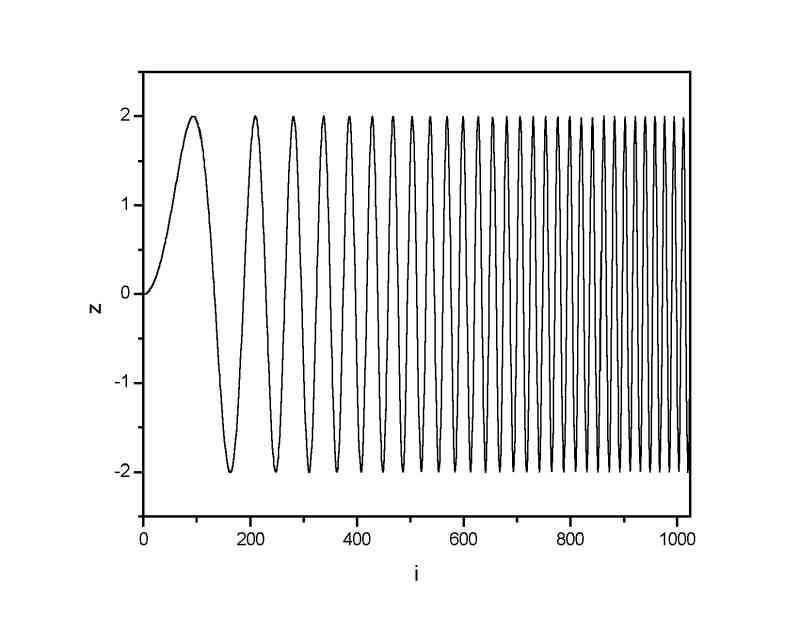
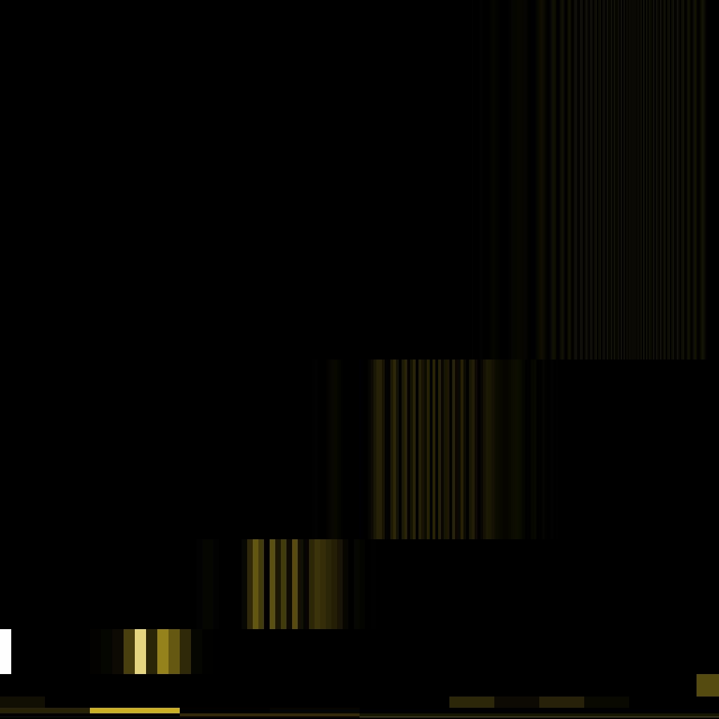
In the next picture a 1024 data long sine signal with linearily increasing frequency. In the next three images there are discrete wavelet spectra obtained using the Haar, Daubechies 4 and Daubechies 20 wavelets as a basis functions.
 |
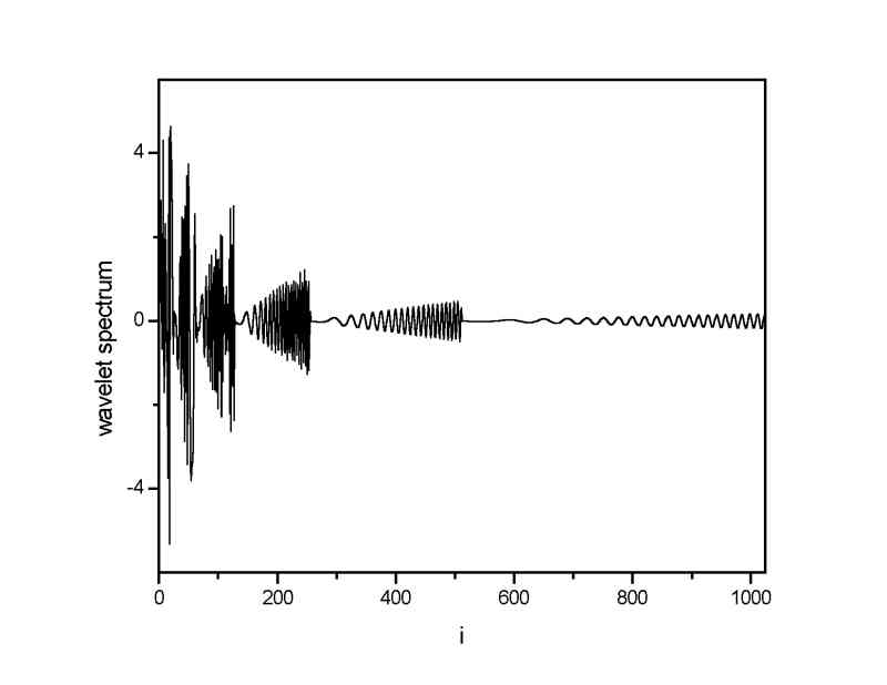 |
| Sine function with increasing frequency. | DWT spectrum using Haar wavelets |
 |
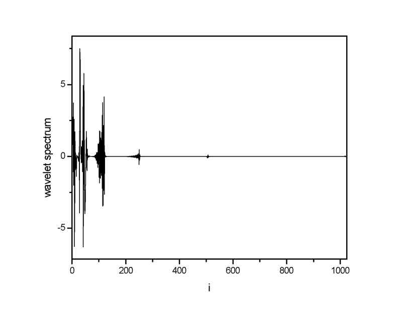 |
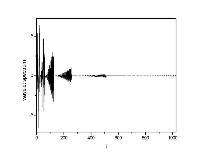
| DWT spectrum using Daubechies 4 wavelets | DWT spectrum using Daubechies 20 wavelets |
From the images one can see that the DWT spectrum obtained using Daubechies 20 wavelets has the lowest number of the non-zero terms (or terms significantly above zero). It is a result of the fact that the Daubechies 20 wavelet is the most continuous one of the wavelets used, and, as it is seen from images of the wavelets, it has a form that is most closed to the sine function. Thus, it is logical that the lowest number of such a wavelets is needed to construct the sine signal.
We can also plot the data obtained by means of DWT to a 2+1D graph similar to the result of the continuous wavelet transform. As there is not enough of data for doing this in the DWT spectra we have to find out first how to fill the time-frequency plane. This is very simple and it reflects the principial uncertainities of the data obdained in wavelet transform. We simply plot the data into a dyadic grid - a grid that consist of tiles of different width and lengt depending on actual time and frequency resolution of each partial DWT spectra component. The signal (sine with power of two increasing frequency) DWT spectrum plotted to a time-frequency plane can be seen at the next image (for comparison there is also a result of continuous wavelet transform using a Morlet wavelet which looks more or less similar to the Daubechies 20 wavelet).
 |
 |
| DWT spectrum plotted into a dyadic grid | Continuous wavelet spectrum computed at the same frequencies approximately |
Created by Petr Klapetek, February 2002