Continuous wavelet transform (CWT) is an implementaion of the wavelet transform using an arbitrary scales and almost arbitrary wavelets. The wavelets used are not orthogonal and the data obtained by this transform are highly correlated. For the disctete time series we can uset this transform as well, with the limitation that the smallest wavelet translations must be equal to the data sampling. This is sometimes called Discrete Time Continuous Wavelet Transform (DT-CWT) and it is the mostly used way of computing CWT in real applications.
In principle the continuous wavelet transform works by using directly the definition of the wavelet transform - e. g. we are computing a convolution of the signal with the scaled wavelet. For each scale we obtain by this way an array of the same length N as the signal has. By using M arbitrarily chosen scales we obtain a field NxM which represents the time-frequency plane directly. The algoritm used for this computaion can be based on a direct convolution or on a convolution by means of multiplication in Fourier space (this is sometimes called Fast wavelet transform).
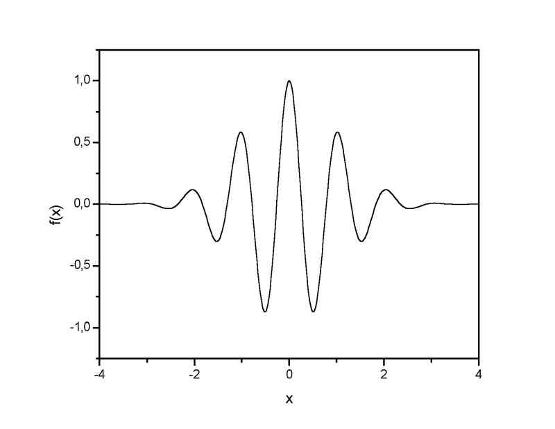
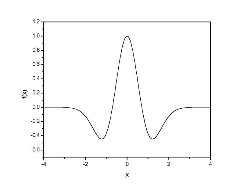
The choice of the wavelet that is used for time-frequency decomposition is the most important thing. By this choice we can infuence the time and frequency resolution of the result. We cannot change the main features of WT by this way (low frequencies have good frequecny and bad time resolution; high frequencies have good time and bad frequency resolution), but we can somehow increase the total frequency of total time resolution. This is directly proportional to the width of the udes wavelet in real and Fourier space. If we use the Morlet wavelet for example (real part - damped cosine function) we can expect high frequency resolution as such a wavelet is very well localized in frequencies. In contrary, using Derivative of Gaussian (DOG) wavelet will result in good time localization, but poor one in frequencies. The Morlet and Derivative of Gaussian wavelets are plotted below.
|
|
| Morlet wavelet (real part) | 2nd. derivative of gaussian wavelet (Mexican hat) |
 |
 |
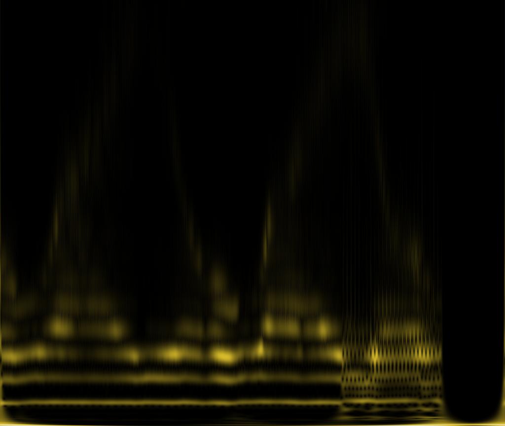
| Signal with increasing and decreasing frequency - the frequency range goes from 50 to 400 Hz | "Vari baba trnku" signal. The syllables are clearly seen as well as the main and higher harmonic frequencies of the sound. The frequency range goes from x to y Hz |
 |
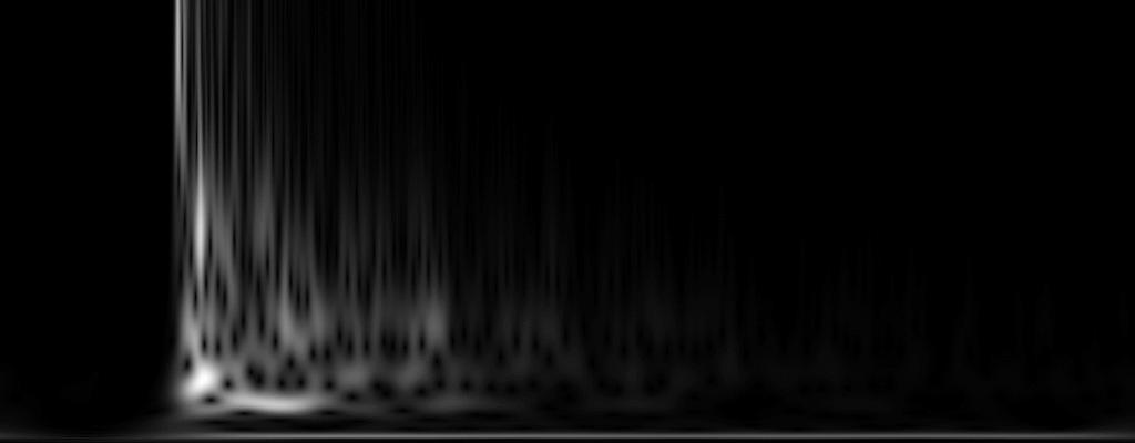 |
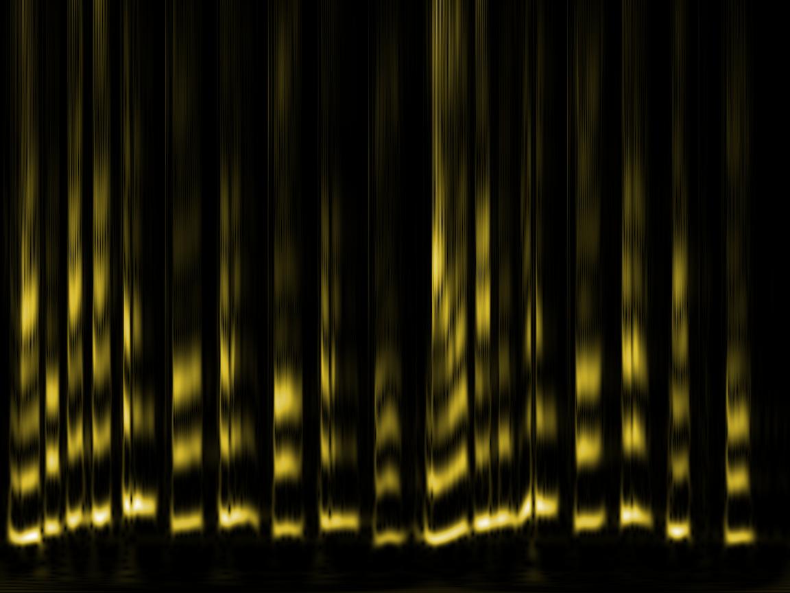
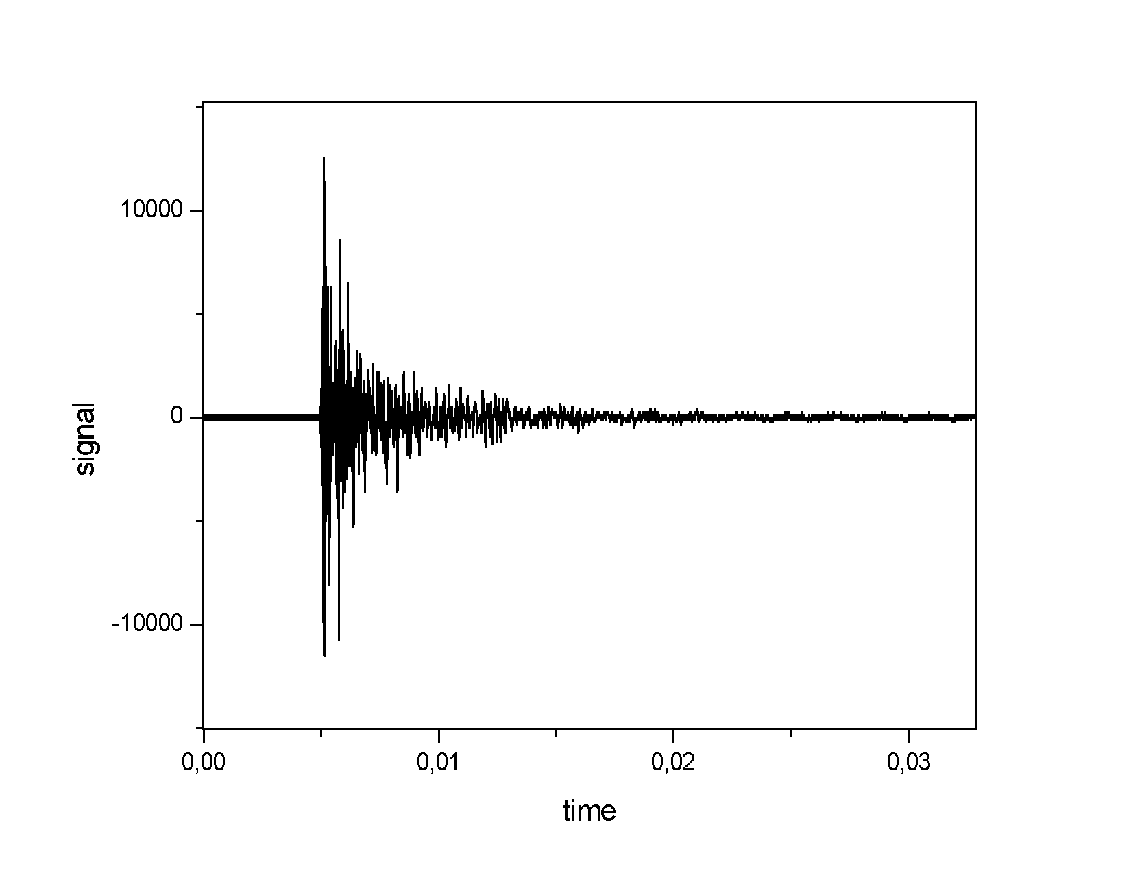
| Hurdiska signal | Hurdiska wavelet spectrum - after the excitation the high frequencies fall down much quickly than the lower ones. There are not any main or base frequencies - the sound is more or less similar to a noise otherwise. The frequency range goes from x to y Hz |
 |
 |
| AEIOU signal CWT spectrum ended with microphone resonance and a piece of silentium. Nevertheless the vowels, each repeated twice (e. g . aeiouaeiou) are clearly different in number and strength of higher harmonics. The base frequency is the same for all the vowels. The frequency range goes from x to y Hz | "Jingle bells" CWT spectrum. The primitive drums and the more or less precise whistle is seen. Listen to the signal if you have doubts. The frequency range goes from x to y Hz |
As it was allredy mentioned, by means of the wavelet choice we can acces different time and frequency resolution in the time-frequency plane. This is demonstrated here for the acoustic emission signal using Morlet, Paul and Mexican hat wavelet.
Not yet...
Created by Petr Klapetek, February 2002